Workshop 1
Exercise 1
Run the following code, then use typeof(), class() functions to find out the data type and/or class object.
my_numeric <- 42.5
John_jay <- "university"
my_logical <- TRUE
my_date <- as.Date("05/29/2018", "%m/%d/%Y")
# for date
typeof(my_date)
#> [1] "double"
class(my_date)
#> [1] "Date"
# for numeric
typeof(my_numeric)
#> [1] "double"
class(my_numeric)
#> [1] "numeric"
# for char
typeof(John_jay)
#> [1] "character"
class(John_jay)
#> [1] "character"
#for logical
typeof(my_logical)
#> [1] "logical"
class(my_logical)
#> [1] "logical"
Exercise 2
Create 1 datatype of each: Character, numeric, integer, complex, Boolean
The answers may vary . Below an example of a solution,
Best_university_in_nyc <- "John Jay"
Best_university_in_nyc
#> [1] "John Jay"
My_gpa <- 3.78
My_gpa
#> [1] 3.78
My_int_gpa <- as.integer(My_gpa)
My_int_gpa
#> [1] 3
my_complex_gpa<- 3.78+2i
my_complex_gpa
#> [1] 3.78+2i
do_I_like_chocolate_ice_cream <- FALSE
do_I_like_chocolate_ice_cream
#> [1] FALSE

my_elements =list(Best_university_in_nyc,My_gpa,My_int_gpa,my_complex_gpa,do_I_like_chocolate_ice_cream)

# Check the classes of each element
for (element in my_elements) {
  print(class(element))
}
#> [1] "character"
#> [1] "numeric"
#> [1] "integer"
#> [1] "complex"
#> [1] "logical"Exercise 1
Exercise 1:
- Create a vector of your favorite numbers.
- Access the third element in your vector.
- Create a new vector that is the square of each element in the original vector.
Create a vector of your favorite numbers.
my_favorite_numbers <- c(7,22,17,19)Access the third element in your vector.
my_favorite_numbers[3]
#> [1] 17
Note that R starts indexing from 1. This is somewhat more natural since we start counting at 1 . However, most programming languages start indexing at 0, that is, to access the third element it would be my_favorite_numbers[2] in a language like python .
Create a new vector that is the square of each element in the original vector.
square_favorite_numbers<- my_favorite_numbers^2
square_favorite_numbers
#> [1]  49 484 289 361
my_vector <- c("Dilan Caro", "Instructor")
names(my_vector) <- c("Name", "Profession")
my_vector
#>         Name   Profession
#> "Dilan Caro" "Instructor"
Inspect my_vector using: the attributes(), the length() and the str() function
attributes(my_vector)
#> $names
#> [1] "Name"       "Profession"
length(my_vector)
#> [1] 2
names(my_vector)
#> [1] "Name"       "Profession"
Exercise 2
- Create a data frame with at least three columns and four rows.
- Print the number of rows and columns of your data frame.
- Display summary statistics of your data frame.
Create a data frame with at least three columns and four rows.
df <- data.frame(
  Subject = c("Art", "Bayesian", "Machine learning", "Stochastic"),
  Grade =c(100,87,90,75),
  Difficulty =c(6,9,8,10)# from 0 to 5 , 5 being the most difficuly
  )
print(df)
#>            Subject Grade Difficulty
#> 1              Art   100          6
#> 2         Bayesian    87          9
#> 3 Machine learning    90          8
#> 4 Stochastic 75 10Exercise 3
Inspect a built-in data frame
mtcars
#>                      mpg cyl  disp  hp drat    wt  qsec vs
#> Mazda RX4           21.0   6 160.0 110 3.90 2.620 16.46  0
#> Mazda RX4 Wag       21.0   6 160.0 110 3.90 2.875 17.02  0
#> Datsun 710          22.8   4 108.0  93 3.85 2.320 18.61  1
#> Hornet 4 Drive      21.4   6 258.0 110 3.08 3.215 19.44  1
#> Hornet Sportabout   18.7   8 360.0 175 3.15 3.440 17.02  0
#> Valiant             18.1   6 225.0 105 2.76 3.460 20.22  1
#> Duster 360          14.3   8 360.0 245 3.21 3.570 15.84  0
#> Merc 240D           24.4   4 146.7  62 3.69 3.190 20.00  1
#> Merc 230            22.8   4 140.8  95 3.92 3.150 22.90  1
#> Merc 280            19.2   6 167.6 123 3.92 3.440 18.30  1
#> Merc 280C           17.8   6 167.6 123 3.92 3.440 18.90  1
#> Merc 450SE          16.4   8 275.8 180 3.07 4.070 17.40  0
#> Merc 450SL          17.3   8 275.8 180 3.07 3.730 17.60  0
#> Merc 450SLC         15.2   8 275.8 180 3.07 3.780 18.00  0
#> Cadillac Fleetwood  10.4   8 472.0 205 2.93 5.250 17.98  0
#> Lincoln Continental 10.4   8 460.0 215 3.00 5.424 17.82  0
#> Chrysler Imperial   14.7   8 440.0 230 3.23 5.345 17.42  0
#> Fiat 128            32.4   4  78.7  66 4.08 2.200 19.47  1
#> Honda Civic         30.4   4  75.7  52 4.93 1.615 18.52  1
#> Toyota Corolla      33.9   4  71.1  65 4.22 1.835 19.90  1
#> Toyota Corona       21.5   4 120.1  97 3.70 2.465 20.01  1
#> Dodge Challenger    15.5   8 318.0 150 2.76 3.520 16.87  0
#> AMC Javelin         15.2   8 304.0 150 3.15 3.435 17.30  0
#> Camaro Z28          13.3   8 350.0 245 3.73 3.840 15.41  0
#> Pontiac Firebird    19.2   8 400.0 175 3.08 3.845 17.05  0
#> Fiat X1-9           27.3   4  79.0  66 4.08 1.935 18.90  1
#> Porsche 914-2       26.0   4 120.3  91 4.43 2.140 16.70  0
#> Lotus Europa        30.4   4  95.1 113 3.77 1.513 16.90  1
#> Ford Pantera L      15.8   8 351.0 264 4.22 3.170 14.50  0
#> Ferrari Dino        19.7   6 145.0 175 3.62 2.770 15.50  0
#> Maserati Bora       15.0   8 301.0 335 3.54 3.570 14.60  0
#> Volvo 142E          21.4   4 121.0 109 4.11 2.780 18.60  1
#>                     am gear carb
#> Mazda RX4            1    4    4
#> Mazda RX4 Wag        1    4    4
#> Datsun 710           1    4    1
#> Hornet 4 Drive       0    3    1
#> Hornet Sportabout    0    3    2
#> Valiant              0    3    1
#> Duster 360           0    3    4
#> Merc 240D            0    4    2
#> Merc 230             0    4    2
#> Merc 280             0    4    4
#> Merc 280C            0    4    4
#> Merc 450SE           0    3    3
#> Merc 450SL           0    3    3
#> Merc 450SLC          0    3    3
#> Cadillac Fleetwood   0    3    4
#> Lincoln Continental  0    3    4
#> Chrysler Imperial    0    3    4
#> Fiat 128             1    4    1
#> Honda Civic          1    4    2
#> Toyota Corolla       1    4    1
#> Toyota Corona        0    3    1
#> Dodge Challenger     0    3    2
#> AMC Javelin          0    3    2
#> Camaro Z28           0    3    4
#> Pontiac Firebird     0    3    2
#> Fiat X1-9            1    4    1
#> Porsche 914-2        1    5    2
#> Lotus Europa         1    5    2
#> Ford Pantera L       1    5    4
#> Ferrari Dino         1    5    6
#> Maserati Bora        1    5    8
#> Volvo 142E           1    4    2
str(mtcars)
#> 'data.frame':    32 obs. of  11 variables:
#>  $ mpg : num  21 21 22.8 21.4 18.7 18.1 14.3 24.4 22.8 19.2 ...
#>  $ cyl : num  6 6 4 6 8 6 8 4 4 6 ...
#>  $ disp: num  160 160 108 258 360 ...
#>  $ hp  : num  110 110 93 110 175 105 245 62 95 123 ...
#>  $ drat: num  3.9 3.9 3.85 3.08 3.15 2.76 3.21 3.69 3.92 3.92 ...
#>  $ wt  : num  2.62 2.88 2.32 3.21 3.44 ...
#>  $ qsec: num  16.5 17 18.6 19.4 17 ...
#>  $ vs  : num  0 0 1 1 0 1 0 1 1 1 ...
#>  $ am  : num  1 1 1 0 0 0 0 0 0 0 ...
#>  $ gear: num  4 4 4 3 3 3 3 4 4 4 ...
#>  $ carb: num  4 4 1 1 2 1 4 2 2 4 ...
head(mtcars)
#>                    mpg cyl disp  hp drat    wt  qsec vs am
#> Mazda RX4         21.0   6  160 110 3.90 2.620 16.46  0  1
#> Mazda RX4 Wag     21.0   6  160 110 3.90 2.875 17.02  0  1
#> Datsun 710        22.8   4  108  93 3.85 2.320 18.61  1  1
#> Hornet 4 Drive    21.4   6  258 110 3.08 3.215 19.44  1  0
#> Hornet Sportabout 18.7   8  360 175 3.15 3.440 17.02  0  0
#> Valiant           18.1   6  225 105 2.76 3.460 20.22  1  0
#>                   gear carb
#> Mazda RX4            4    4
#> Mazda RX4 Wag        4    4
#> Datsun 710           4    1
#> Hornet 4 Drive       3    1
#> Hornet Sportabout    3    2
#> Valiant              3    1
Get summary from a variable in a dataframe
summary(mtcars$cyl) # use $ to extract variable from a data frame
#>    Min. 1st Qu.  Median    Mean 3rd Qu.    Max.
#>   4.000   4.000   6.000   6.188   8.000   8.000
Now inspect a tibble
library(ggplot2)
diamonds
#> # A tibble: 53,940 × 10
#>    carat cut     color clarity depth table price     x     y
#>    <dbl> <ord>   <ord> <ord>   <dbl> <dbl> <int> <dbl> <dbl>
#>  1  0.23 Ideal   E     SI2      61.5    55   326  3.95  3.98
#>  2  0.21 Premium E     SI1      59.8    61   326  3.89  3.84
#>  3  0.23 Good    E     VS1      56.9    65   327  4.05  4.07
#>  4  0.29 Premium I     VS2      62.4    58   334  4.2   4.23
#>  5  0.31 Good    J     SI2      63.3    58   335  4.34  4.35
#>  6  0.24 Very G… J     VVS2     62.8    57   336  3.94  3.96
#>  7  0.24 Very G… I     VVS1     62.3    57   336  3.95  3.98
#>  8  0.26 Very G… H     SI1      61.9    55   337  4.07  4.11
#>  9  0.22 Fair    E     VS2      65.1    61   337  3.87  3.78
#> 10  0.23 Very G… H     VS1      59.4    61   338  4     4.05
#> # ℹ 53,930 more rows
#> # ℹ 1 more variable: z <dbl>
str(diamonds)  # built-in in library ggplot2
#> tibble [53,940 × 10] (S3: tbl_df/tbl/data.frame)
#>  $ carat  : num [1:53940] 0.23 0.21 0.23 0.29 0.31 0.24 0.24 0.26 0.22 0.23 ...
#>  $ cut    : Ord.factor w/ 5 levels "Fair"<"Good"<..: 5 4 2 4 2 3 3 3 1 3 ...
#>  $ color  : Ord.factor w/ 7 levels "D"<"E"<"F"<"G"<..: 2 2 2 6 7 7 6 5 2 5 ...
#>  $ clarity: Ord.factor w/ 8 levels "I1"<"SI2"<"SI1"<..: 2 3 5 4 2 6 7 3 4 5 ...
#>  $ depth  : num [1:53940] 61.5 59.8 56.9 62.4 63.3 62.8 62.3 61.9 65.1 59.4 ...
#>  $ table  : num [1:53940] 55 61 65 58 58 57 57 55 61 61 ...
#>  $ price  : int [1:53940] 326 326 327 334 335 336 336 337 337 338 ...
#>  $ x      : num [1:53940] 3.95 3.89 4.05 4.2 4.34 3.94 3.95 4.07 3.87 4 ...
#>  $ y      : num [1:53940] 3.98 3.84 4.07 4.23 4.35 3.96 3.98 4.11 3.78 4.05 ...
#>  $ z      : num [1:53940] 2.43 2.31 2.31 2.63 2.75 2.48 2.47 2.53 2.49 2.39 ...
head(diamonds)
#> # A tibble: 6 × 10
#>   carat cut      color clarity depth table price     x     y
#>   <dbl> <ord>    <ord> <ord>   <dbl> <dbl> <int> <dbl> <dbl>
#> 1  0.23 Ideal    E     SI2      61.5    55   326  3.95  3.98
#> 2  0.21 Premium  E     SI1      59.8    61   326  3.89  3.84
#> 3  0.23 Good     E     VS1      56.9    65   327  4.05  4.07
#> 4  0.29 Premium  I     VS2      62.4    58   334  4.2   4.23
#> 5  0.31 Good     J     SI2      63.3    58   335  4.34  4.35
#> 6  0.24 Very Go… J     VVS2     62.8    57   336  3.94  3.96
#> # ℹ 1 more variable: z <dbl>
summary(diamonds$depth)
#>    Min. 1st Qu.  Median    Mean 3rd Qu.    Max.
#>   43.00   61.00   61.80   61.75   62.50   79.00
Exercise 4
- Create a vector
fav_musicwith the names of your favorite artists. - Create a vector
num_recordswith the number of records you have in your collection of each of those artists. - Create a vector
num_concertswith the number of times you attended a concert of these artists. - Put everything together in a data frame, assign the name
my_musicto this data frame and change the labels of the information stored in the columns toartist,recordsandconcerts. - Extract the variable
num_recordsfrom the data framemy_music. - Calculate the total number of records in your collection (for the defined set of artists).
- Check the structure of the data frame, ask for a
summary.
fav_music <- c("Prince", "REM", "Ryan Adams", "BLOF")
num_concerts <- c(0, 3, 1, 0)
num_records <- c(2, 7, 5, 1)
my_music <- data.frame(fav_music, num_concerts, num_records)
names(my_music) <- c("artist", "concerts", "records")
summary(my_music)
#>     artist             concerts      records
#>  Length:4           Min.   :0.0   Min.   :1.00
#>  Class :character   1st Qu.:0.0   1st Qu.:1.75
#>  Mode  :character   Median :0.5   Median :3.50
#>                     Mean   :1.0   Mean   :3.75
#>                     3rd Qu.:1.5   3rd Qu.:5.50
#>                     Max.   :3.0   Max.   :7.00
my_music$records
#> [1] 2 7 5 1
sum(my_music$records)
#> [1] 15
Import other data formats
The haven package enables R to read and write various data formats used by other statistical packages.
It supports:
- SAS:
read_sas()reads .sas7bdat and .sas7bcat files andread_xpt()reads SAS transport files. write_sas() writes .sas7bdat files. - SPSS:
read_sav()reads .sav files andread_por()reads the older .por files. write_sav() writes .sav files. - Stata:
read_dta()reads .dta files.write_dta()writes .dta files.
Exercise 5
Load the following data sets, available in the course material:
- the Danish fire insurance losses, stored in danish.txt
- the severity data set, stored in severity.sas7bdat.
path <- file.path('/Users/dilancaro/Library/Mobile Documents/com~apple~CloudDocs/Workshops/John Jay/R Workshop/R-workshop-John-Jay/John Jay Workshop Data/')
path.danish <- file.path(path, "danish.txt")
danish <- read.table(path.danish, header = TRUE)
danish$Date <- as.Date(danish$Date, "%m/%d/%Y")
str(danish)
#> 'data.frame':    2167 obs. of  2 variables:
#>  $ Date       : Date, format: "1980-01-03" ...
#>  $ Loss.in.DKM: num  1.68 2.09 1.73 1.78 4.61 ...
library(haven)
severity <- read_sas('/Users/dilancaro/Library/Mobile Documents/com~apple~CloudDocs/Workshops/John Jay/R Workshop/R-workshop-John-Jay/John Jay Workshop Data/severity.sas7bdat')
str(severity)
#> tibble [19,287 × 5] (S3: tbl_df/tbl/data.frame)
#>  $ policyId   : num [1:19287] 6e+05 6e+05 6e+05 6e+05 6e+05 ...
#>   ..- attr(*, "format.sas")= chr "BEST"
#>  $ claimId    : num [1:19287] 9e+05 9e+05 9e+05 9e+05 9e+05 ...
#>   ..- attr(*, "format.sas")= chr "BEST"
#>  $ rc         : num [1:19287] 35306 19773 41639 10649 20479 ...
#>   ..- attr(*, "format.sas")= chr "BEST"
#>  $ deductible : num [1:19287] 1200 50 100 50 50 50 50 50 50 50 ...
#>   ..- attr(*, "format.sas")= chr "BEST"
#>  $ claimAmount: num [1:19287] 35306 19773 41639 10649 20479 ...
#> ..- attr(*, "format.sas")= chr "COMMA"Exercises
- Subsetting Data Frames
Create a data frame named student_info with the following columns and data: - student_id (1 to 5) - student_name (‘Alice’, ‘Bob’, ‘Charlie’, ‘David’, ‘Eva’) - student_age (25, 30, 22, 28, 24) - student_grade (‘A’, ‘B’, ‘A’, ‘C’, ‘B’)
Write a command to subset this data frame to include only students older than 24.
- Using Conditional Filters
- Use the subset() function to find all students with a grade of ‘A’.
- Display the names and ages of these students.
- Manipulating Data with dplyr
Load the dplyr package and convert student_info to a tibble.
Use filter() and select() to show the name and age of students who have a grade better than ‘B’.
- Adding and Removing Columns
- Add a new column student_major with values (‘Math’, ‘Science’, ‘Arts’, ‘Math’, ‘Science’) to student_info.
- Then, remove the student_grade column using dplyr.
- Renaming Columns
- Rename the student_name column to name using base R functions and then using dplyr.
- Complex dplyr Operations
- Create a new tibble from student_info that includes all students except those studying ‘Arts’, rename the student_id column to id, and arrange the students by age in descending order.
- Exploratory Data Analysis with dplyr
- Calculate the average age of students grouped by their major using group_by() and summarize() in dplyr.
# Exercise 1: Subsetting Data Frames
student_info <- data.frame(
  student_id = 1:5,
  student_name = c("Alice", "Bob", "Charlie", "David", "Eva"),
  student_age = c(25, 30, 22, 28, 24),
  student_grade = c('A', 'B', 'A', 'C', 'B')
)
older_students <- subset(student_info, student_age > 24)
# Exercise 2: Using Conditional Filters

grade_a_students <- subset(student_info, student_grade == 'A', select = c(student_name, student_age))
# Exercise 3: Manipulating Data with dplyr
library(dplyr)
#>
#> Attaching package: 'dplyr'
#> The following objects are masked from 'package:stats':
#>
#>     filter, lag
#> The following objects are masked from 'package:base':
#>
#>     intersect, setdiff, setequal, union
student_info <- as_tibble(student_info)
good_students <- student_info %>% filter(student_grade > 'B') %>% select(student_name, student_age)
# Exercise 4: Adding and Removing Columns
student_info <- mutate(student_info, student_major = c('Math', 'Science', 'Arts', 'Math', 'Science'))
student_info <- select(student_info, -student_grade)
# Exercise 5: Renaming Columns
student_info <- data.frame(
  student_id = 1:5,
  student_name = c("Alice", "Bob", "Charlie", "David", "Eva"),
  student_age = c(25, 30, 22, 28, 24),
  student_grade = c('A', 'B', 'A', 'C', 'B')
)

names(student_info)[names(student_info) == "student_name"] <- "name"

student_info <- data.frame(
  student_id = 1:5,
  student_name = c("Alice", "Bob", "Charlie", "David", "Eva"),
  student_age = c(25, 30, 22, 28, 24),
  student_grade = c('A', 'B', 'A', 'C', 'B')
)
student_info <- rename(student_info, name = student_name)
student_info <- data.frame(
  student_id = 1:5,
  student_name = c("Alice", "Bob", "Charlie", "David", "Eva"),
  student_age = c(25, 30, 22, 28, 24),
  student_grade = c('A', 'B', 'A', 'C', 'B')
)

# Exercise 6: Complex dplyr Operations
student_info <- mutate(student_info, student_major = c('Math', 'Science', 'Arts', 'Math', 'Science'))
student_info <- select(student_info, -student_grade)

filtered_info <- student_info %>%
  filter(student_major != "Arts") %>%
  rename(id = student_id) %>%
arrange(desc(student_age))Part V
Exercise 1
Making a Scatter plot:
- load the journals.txt data set and save as Journals data frame
- Work through the following instructions
Journals<-read.table("~/Library/Mobile Documents/com~apple~CloudDocs/Workshops/John Jay/R Workshop/R-workshop-John-Jay/John Jay Workshop Data/journals.txt")

str(Journals)
#> 'data.frame':    180 obs. of  10 variables:
#>  $ title       : chr  "Asian-Pacific Economic Literature" "South African Journal of Economic History" "Computational Economics" "MOCT-MOST Economic Policy in Transitional Economics" ...
#>  $ publisher   : chr  "Blackwell" "So Afr ec history assn" "Kluwer" "Kluwer" ...
#>  $ society     : chr  "no" "no" "no" "no" ...
#>  $ price       : int  123 20 443 276 295 344 90 242 226 262 ...
#>  $ pages       : int  440 309 567 520 791 609 602 665 243 386 ...
#>  $ charpp      : int  3822 1782 2924 3234 3024 2967 3185 2688 3010 2501 ...
#>  $ citations   : int  21 22 22 22 24 24 24 27 28 30 ...
#>  $ foundingyear: int  1986 1986 1987 1991 1972 1994 1995 1968 1987 1949 ...
#>  $ subs        : int  14 59 17 2 96 15 14 202 46 46 ...
#>  $ field       : chr  "General" "Economic History" "Specialized" "Area Studies" ...
plot(log(Journals$subs), log(Journals$price))
rug(log(Journals$subs))
rug(log(Journals$price), side = 2)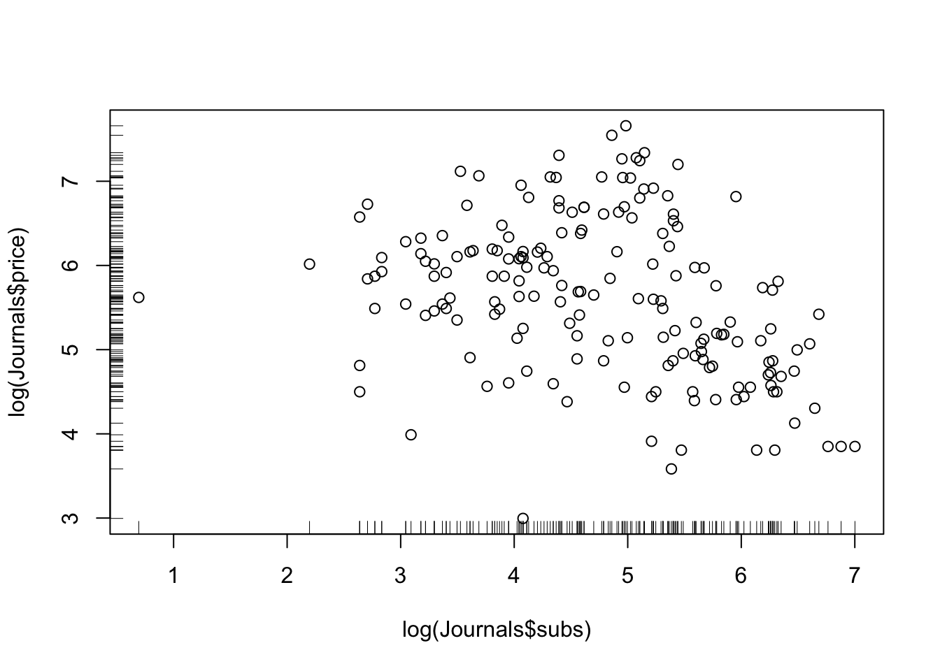
plot(log(Journals$price) ~ log(Journals$subs), pch = 19,
     col = "blue", xlim = c(0, 7), ylim = c(3, 8),
     main = "Library subscriptions")
rug(log(Journals$subs))
rug(log(Journals$price), side=2)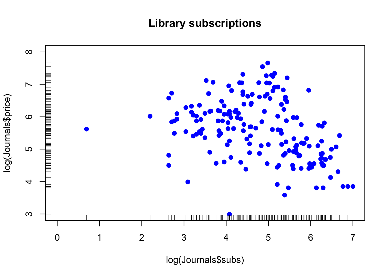
Exercise 2
Now, try creating your own visualization using the iris dataset. Here’s what you can do:
- Create a scatter plot using Petal.Length and Petal.Width from the iris dataset.
- Color the points based on the Species column to differentiate between the species.
- Add a title, x-axis label, and y-axis label to your plot. Include a legend that indicates which color corresponds to which iris species.
data(iris)
# Create the scatter plot
plot(iris$Petal.Length, iris$Petal.Width, col=as.factor(iris$Species),
main="Iris Petal Measurements",
xlab="Petal Length", ylab="Petal Width",
pch=19)
# Add a legend
legend("topright", legend=levels(iris$Species), col=1:length(levels(iris$Species)), pch=19)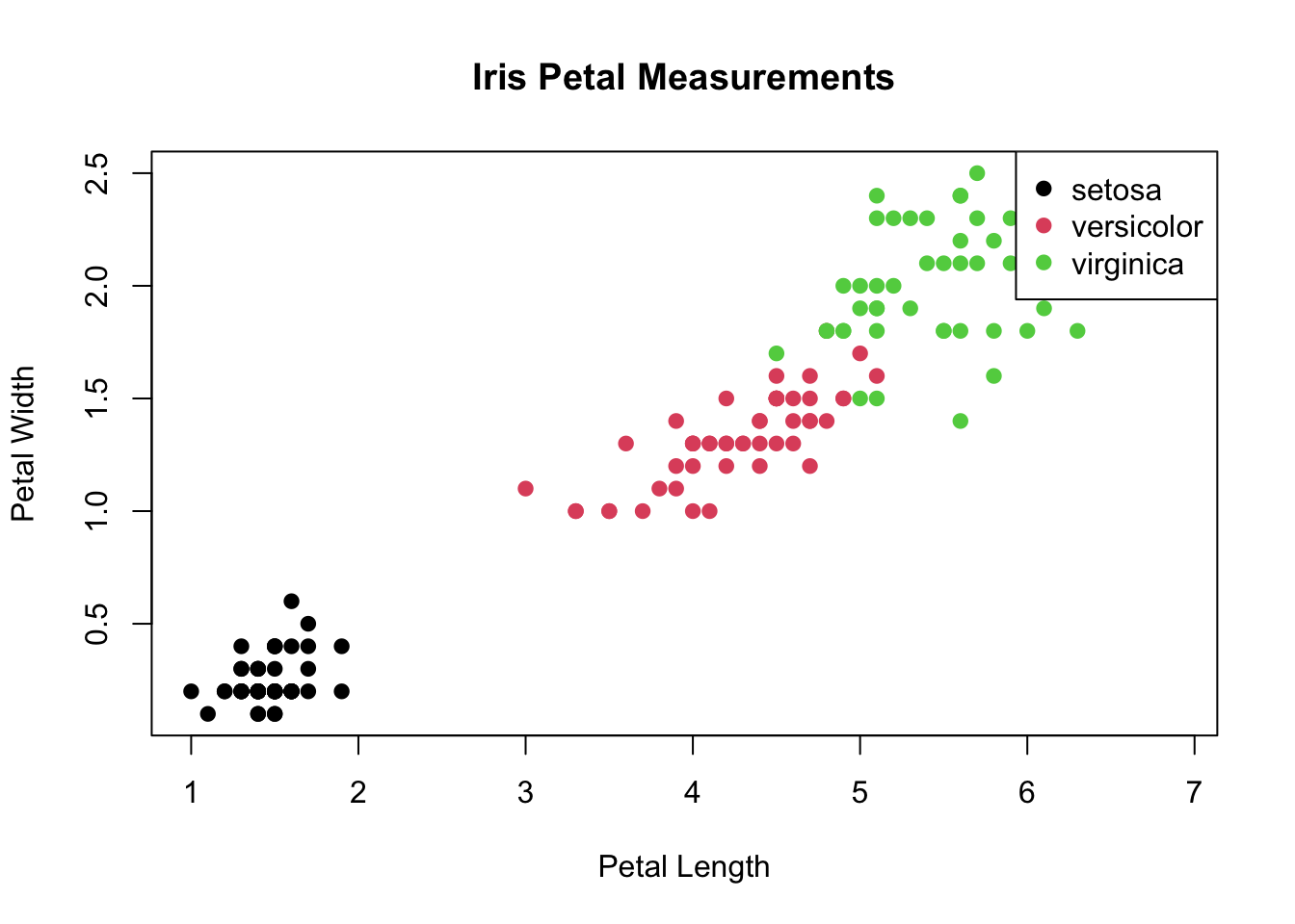 ## Example 4 {-}
Explanation:
iris$Sepal.Length: This selects the Sepal.Length column from the iris dataset as the x-coordinates for the plot.
iris$Sepal.Width: This selects the Sepal.Width column from the iris dataset as the y-coordinates for the plot.
col=iris$Species: This assigns colors to the points based on the Species column, which means that each species will have a different color in the plot.
main: Sets the title of the plot to “Iris Sepal Measurements”.
xlab: Sets the label for the x-axis to “Sepal Length”.
ylab: Sets the label for the y-axis to “Sepal Width”.
pch=19: Sets the plotting character (or point symbol) to a solid circle.