Part III: Data Structures

Vectors: Creating, indexing, and operations

# Creating a vector
v <- c(1, 2, 3, 4, 5)
print(v)
#> [1] 1 2 3 4 5

# Indexing a vector
print(v[2])  # Access the second element
#> [1] 2

# Vector operations
v2 <- v * 2  # Multiply each element by 2
print(v2)
#> [1]  2  4  6  8 10

You can give names to the columns of the vector

my_vector <- c("Dilan Caro", "Instructor")
names(my_vector) <- c("Name", "Profession")
my_vector
#>         Name   Profession 
#> "Dilan Caro" "Instructor"

Exercise 1:

Create a vector of your favorite numbers.
Access the third element in your vector.
Create a new vector that is the square of each element in the original vector.

my_vector <- c("Dilan Caro", "Instructor")
names(my_vector) <- c("Name", "Profession")
my_vector
#>         Name   Profession 
#> "Dilan Caro" "Instructor"

Inspect my_vector using: the attributes(), the length() and the str() function

Matrices

Matrices are vectors with a dimension attribute. The dimension attribute is itself an integer vector of length 2 (number of rows, number of columns)

Matrices are constructed column-wise, so entries can be thought of starting in the “upper left” corner and running down the columns.

m <- matrix(1:6, nrow = 2, ncol = 3) 
m
#>      [,1] [,2] [,3]
#> [1,]    1    3    5
#> [2,]    2    4    6

Another example

my_matrix <- matrix(1:12, 3, 4, byrow = TRUE)
my_matrix
#>      [,1] [,2] [,3] [,4]
#> [1,]    1    2    3    4
#> [2,]    5    6    7    8
#> [3,]    9   10   11   12

Matrices can be created by column-binding or row-binding with the cbind() and rbind() functions.

x <- 1:3
y <- 10:12
cbind(x, y)
#>      x  y
#> [1,] 1 10
#> [2,] 2 11
#> [3,] 3 12
rbind(x, y)
#>   [,1] [,2] [,3]
#> x    1    2    3
#> y   10   11   12

Seq and rep functions

In R, seq and rep are two functions used to generate sequences and to replicate values, respectively.

0.0.1 `seq` Function:

The seq function is used to create a sequence of numbers.

Usage:

seq(from, to): Generates a sequence from the ‘from’ value to the ‘to’ value with a default increment of 1.
seq(from, to, by): Generates a sequence from the ‘from’ value to the ‘to’ value, with the increment specified by ‘by’.
seq(from, to, length.out): Generates a sequence from the ‘from’ value to the ‘to’ value with a specified number of equally spaced points.

Example

seq(1, 5)         
#> [1] 1 2 3 4 5
seq(1, 10, by = 2)    
#> [1] 1 3 5 7 9
seq(1, 10, length.out = 4) 
#> [1]  1  4  7 10

0.0.2 `rep` Function:

The rep function is used to replicate the values in a vector.

Usage:

rep(x, times): Replicates each element in ‘x’ a specified number of ‘times’.
rep(x, each): Replicates each element in ‘x’ ‘each’ times before moving to the next element.
rep(x, length.out): Replicates the values in ‘x’ up to the ‘length.out’ number of times in total.

rep(1:3, times = 2)
#> [1] 1 2 3 1 2 3
rep(1:3, each = 2)       
#> [1] 1 1 2 2 3 3
rep(1:3, length.out = 7)   
#> [1] 1 2 3 1 2 3 1

Lists

Lists are a special type of vector that can contain elements of different classes. Lists are a very important data type in R and you should get to know them well. Lists, in combination with the various “apply” functions discussed later, make for a powerful combination.

Lists can be explicitly created using the list() function, which takes an arbitrary number of arguments.

x <- list(1, "a", TRUE, 1 + 4i) 
x
#> [[1]]
#> [1] 1
#> 
#> [[2]]
#> [1] "a"
#> 
#> [[3]]
#> [1] TRUE
#> 
#> [[4]]
#> [1] 1+4i

Example

my_list <- list(one = 1, two = c(1, 2), five = seq(1, 4, length=5),
          six = c("Dilan", "April"))
names(my_list)
#> [1] "one"  "two"  "five" "six"

str(my_list)
#> List of 4
#>  $ one : num 1
#>  $ two : num [1:2] 1 2
#>  $ five: num [1:5] 1 1.75 2.5 3.25 4
#>  $ six : chr [1:2] "Dilan" "April"

Factors

Factors are used to represent categorical data and can be unordered or ordered. One can think of a factor as an integer vector where each integer has a label. Factors are important in statistical modeling and are treated specially by modelling functions like lm() and glm().

Using factors with labels is better than using integers because factors are self-describing. Having a variable that has values “Male” and “Female” is better than a variable that has values 1 and 2.

Factor objects can be created with the factor() function.

x <- factor(c("yes", "yes", "no", "yes", "no")) 
x
#> [1] yes yes no  yes no 
#> Levels: no yes

Level are put in alphabetical order, but you can also define the levels.

x <- factor(c("yes", "yes", "no", "yes", "no"),levels = c("yes", "no"))
x
#> [1] yes yes no  yes no 
#> Levels: yes no

Data frames: Creating and exploring data frames

Data frames are used to store tabular data in R.

Data frames are represented as a special type of list where every element of the list has to have the same length. Each element of the list can be thought of as a column and the length of each element of the list is the number of rows.

# Creating a data frame
df <- data.frame(
  Name = c("Alice", "Bob", "Charlie"),
  Age = c(25, 30, 35),
  Salary = c(50000, 60000, 70000)
)
print(df)
#>      Name Age Salary
#> 1   Alice  25  50000
#> 2     Bob  30  60000
#> 3 Charlie  35  70000

# Exploring data frames
print(dim(df))  # Dimensions of the data frame
#> [1] 3 3
print(colnames(df))  # Column names
#> [1] "Name"   "Age"    "Salary"
print(summary(df))  # Summary statistics
#>      Name                Age           Salary     
#>  Length:3           Min.   :25.0   Min.   :50000  
#>  Class :character   1st Qu.:27.5   1st Qu.:55000  
#>  Mode  :character   Median :30.0   Median :60000  
#>                     Mean   :30.0   Mean   :60000  
#>                     3rd Qu.:32.5   3rd Qu.:65000  
#>                     Max.   :35.0   Max.   :70000

Exercise 2

Create a data frame with at least three columns and four rows.
Print the number of rows and columns of your data frame.
Display summary statistics of your data frame.

Part 2

Exercise 3

Inspect a built-in data frame, inspect mtcars using str(), head()
Get summary from a variable in a dataframe, use $ to extract a variable from the dataframe.
Now inspect a tibble, inspect diamonds from the ggplot2 library. Use str(), head(), summary()

mtcars
str(mtcars)
head(mtcars)

summary(mtcars$cyl) # use $ to extract variable from a data frame

library(ggplot2)
head(diamonds)

Can you list some differences?

Importing and exporting data (CSV files)

Exporting data to CSV

write.csv(df, "my_data.csv", row.names = FALSE)

Importing data from CSV

df_imported <- read.csv("my_data.csv")
print(df_imported)
#>      Name Age Salary
#> 1   Alice  25  50000
#> 2     Bob  30  60000
#> 3 Charlie  35  70000

Exercise 4

Create a vector fav_music with the names of your favorite artists.
Create a vector num_records with the number of records you have in your collection of each of those artists.
Create a vector num_concerts with the number of times you attended a concert of these artists.
Put everything together in a data frame, assign the name my_music to this data frame and change the labels of the information stored in the columns to artist, records and concerts.
Extract the variable num_records from the data frame my_music.
Calculate the total number of records in your collection (for the defined set of artists).
Check the structure of the data frame, ask for a summary.

Previously, we exported the data and then imported it . Some of you may think, then what is the purpose if we already had the dataframe. The prior was just an example, in reality , you would not have the dataframe loaded in R . You would only have a csv or a data file that a coworker has shared with you or the data engineer has procured for you.

First, we need to obtain the data that we need. For that, please head over to

https://tinyurl.com/JJAY-R-workshop

alternatively,

https://drive.google.com/drive/folders/18W5f2AvKT7IVKnJ73McCzQOOqMdP0CwM?usp=sharing

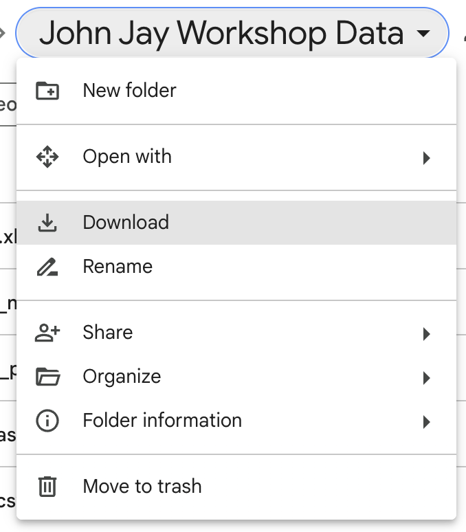
Download the data, for that, click on the arrow of the folder, and choose download. Find where it is located in your computer, obtain the Path

Some useful instructions regarding path names: get your working directory

Get working directory

getwd()
#> [1] "/Users/dilancaro/Library/Mobile Documents/com~apple~CloudDocs/Workshops/John Jay/R Workshop/R-workshop-John-Jay"

specify a path name, with forward slash or double back slash

path <- file.path("/Users/dilancaro/Library/Mobile Documents/com~apple~CloudDocs/Workshops/John Jay/R Workshop/R-workshop-John-Jay/John Jay Workshop Data")

use a relative path

path <- file.path("./John Jay Workshop Data")

Importing a .txt file

read.table() is one great way to import data.


path.hotdogs <- file.path(path, "hotdogs.txt")
path.hotdogs    # inspect path name
#> [1] "./John Jay Workshop Data/hotdogs.txt"
hotdogs <- read.table(path.hotdogs, header = FALSE,
                      col.names = c("type", "calories", "sodium"))
str(hotdogs)    # inspect data imported
#> 'data.frame':    54 obs. of  3 variables:
#>  $ type    : chr  "Beef" "Beef" "Beef" "Beef" ...
#>  $ calories: int  186 181 176 149 184 190 158 139 175 148 ...
#>  $ sodium  : int  495 477 425 322 482 587 370 322 479 375 ...

Or like this

hotdogs2 <- read.table(path.hotdogs, header = FALSE,
                       col.names = c("type", "calories", "sodium"),
                       colClasses = c("factor", "NULL", "numeric"))
str(hotdogs2)
#> 'data.frame':    54 obs. of  2 variables:
#>  $ type  : Factor w/ 3 levels "Beef","Meat",..: 1 1 1 1 1 1 1 1 1 1 ...
#>  $ sodium: num  495 477 425 322 482 587 370 322 479 375 ...

What happened?

Import .csv file

read.csv() is another importing function.

Here is an example: - load a data set on swimming pools in Brisbane - column names in the first row; a comma to separate values within rows

path.pools <- file.path(path, "swimming_pools.csv")
pools <- read.csv(path.pools)
str(pools)
#> 'data.frame':    20 obs. of  4 variables:
#>  $ Name     : chr  "Acacia Ridge Leisure Centre" "Bellbowrie Pool" "Carole Park" "Centenary Pool (inner City)" ...
#>  $ Address  : chr  "1391 Beaudesert Road, Acacia Ridge" "Sugarwood Street, Bellbowrie" "Cnr Boundary Road and Waterford Road Wacol" "400 Gregory Terrace, Spring Hill" ...
#>  $ Latitude : num  -27.6 -27.6 -27.6 -27.5 -27.4 ...
#>  $ Longitude: num  153 153 153 153 153 ...

Import .xlsx file

The package to read excel data into R is readxl:

No external dependencies, easy to download
Desgined to work with tabular data

library(readxl)
path.urbanpop <- file.path(path, "urbanpop.xlsx")
excel_sheets(path.urbanpop) # list sheet names with excel_sheets()
#> [1] "1960-1966" "1967-1974" "1975-2011"

Specify a worksheet by name or number, e.g.

pop_1 <- read_excel(path.urbanpop, sheet = 1)
pop_2 <- read_excel(path.urbanpop, sheet = 2)

inspect and re-combine

str(pop_1)
#> tibble [209 × 8] (S3: tbl_df/tbl/data.frame)
#>  $ country: chr [1:209] "Afghanistan" "Albania" "Algeria" "American Samoa" ...
#>  $ 1960   : num [1:209] 769308 494443 3293999 NA NA ...
#>  $ 1961   : num [1:209] 814923 511803 3515148 13660 8724 ...
#>  $ 1962   : num [1:209] 858522 529439 3739963 14166 9700 ...
#>  $ 1963   : num [1:209] 903914 547377 3973289 14759 10748 ...
#>  $ 1964   : num [1:209] 951226 565572 4220987 15396 11866 ...
#>  $ 1965   : num [1:209] 1000582 583983 4488176 16045 13053 ...
#>  $ 1966   : num [1:209] 1058743 602512 4649105 16693 14217 ...
pop_list <- list(pop_1, pop_2)

Import other data formats

The haven package enables R to read and write various data formats used by other statistical packages.

It supports:

SAS: read_sas() reads .sas7bdat and .sas7bcat files and read_xpt() reads SAS transport files. write_sas() writes .sas7bdat files.
SPSS: read_sav() reads .sav files and read_por() reads the older .por files. write_sav() writes .sav files.
Stata: read_dta() reads .dta files. write_dta() writes .dta files.

0.1 Create and format dates

To create a Date object from a simple character string in R, you can use the as.Date() function. The character string has to obey a format that can be defined using a set of symbols (the examples correspond to 13 January, 1982):

%Y: 4-digit year (1982) %y: 2-digit year (82) %m: 2-digit month (01) %d: 2-digit day of the month (13) %A: weekday (Wednesday) %a: abbreviated weekday (Wed) %B: month (January) %b: abbreviated month (Jan)

Exercise 5

Load the following data sets, available in the course material: - the Danish fire insurance losses, stored in danish.txt - the severity data set, stored in severity.sas7bdat.

Part II: R Fundamentals

Part IV: Data Manipulation

Part III: Data Structures

Vectors: Creating, indexing, and operations

Exercise 1:

Matrices

Seq and rep functions

0.0.1 seq Function:

Example

0.0.2 rep Function:

Lists

Example

Factors

Data frames: Creating and exploring data frames

Exercise 2

Part 2

Exercise 3

Importing and exporting data (CSV files)

Exercise 4

Importing a .txt file

Import .csv file

Import .xlsx file

Import other data formats

0.1 Create and format dates

Exercise 5

0.0.1 `seq` Function:

0.0.2 `rep` Function: