Part II: Statistical Analysis
Introduction to hypothesis testing and statistical tests
Hypothesis testing is a statistical method used to make inferences or draw conclusions about a population based on sample data. It starts with a null hypothesis (H0) that assumes no effect or no difference, and an alternative hypothesis (H1) that contradicts the null hypothesis.
The process involves: 1. Defining the null and alternative hypotheses.
Selecting a significance level (alpha, typically 0.05).
Calculating a test statistic based on the sample data.
Determining the p-value, which is the probability of observing the test statistic or something more extreme under the null hypothesis.
Comparing the p-value with the significance level to decide whether to reject the null hypothesis.
Statistical tests vary based on the type of data and the research question. Common tests include t-tests (for means), chi-squared tests (for categorical data), ANOVA (for comparing means across multiple groups), and regression analysis (for relationships between variables).
0.2 Comparing Variances
- F test to compare variances (Parametric)
x <- rnorm(50, mean = 0, sd = 2)
y <- rnorm(30, mean = 1, sd = 1)
var.test(x, y)
#>
#>  F test to compare two variances
#>
#> data:  x and y
#> F = 4.6796, num df = 49, denom df = 29, p-value =
#> 3.149e-05
#> alternative hypothesis: true ratio of variances is not equal to 1
#> 95 percent confidence interval:
#>  2.351119 8.804199
#> sample estimates:
#> ratio of variances
#> 4.679559- Barlett test: Testing homogeneity (Parametric)
Performs Bartlett’s test of the null that the variances in each of the groups (samples) are the same.
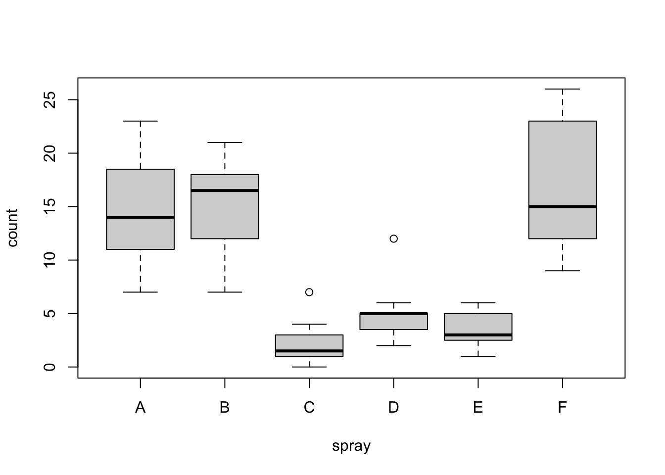
bartlett.test(InsectSprays$count, InsectSprays$spray)
#>
#>  Bartlett test of homogeneity of variances
#>
#> data:  InsectSprays$count and InsectSprays$spray
#> Bartlett's K-squared = 25.96, df = 5, p-value =
#> 9.085e-05- Fligner-Killeen Test of Homogeneity of Variances (Non-parametric)
fligner.test(InsectSprays$count, InsectSprays$spray)
#>
#>  Fligner-Killeen test of homogeneity of variances
#>
#> data:  InsectSprays$count and InsectSprays$spray
#> Fligner-Killeen:med chi-squared = 14.483, df = 5,
#> p-value = 0.01282- Mood Two-Sample Test of Scale (Non-Parametric)
ramsay <- c(111, 107, 100, 99, 102, 106, 109, 108, 104, 99,
            101, 96, 97, 102, 107, 113, 116, 113, 110, 98)
jung.parekh <- c(107, 108, 106, 98, 105, 103, 110, 105, 104,
            100, 96, 108, 103, 104, 114, 114, 113, 108, 106, 99)
mood.test(ramsay, jung.parekh)
#>
#>  Mood two-sample test of scale
#>
#> data:  ramsay and jung.parekh
#> Z = 1.0371, p-value = 0.2997
#> alternative hypothesis: two.sided- Ansari-Bradley Test (Non-parametric)
ramsay <- c(111, 107, 100, 99, 102, 106, 109, 108, 104, 99,
            101, 96, 97, 102, 107, 113, 116, 113, 110, 98)
jung.parekh <- c(107, 108, 106, 98, 105, 103, 110, 105, 104,
            100, 96, 108, 103, 104, 114, 114, 113, 108, 106, 99)
ansari.test(ramsay, jung.parekh)
#> Warning in ansari.test.default(ramsay, jung.parekh): cannot
#> compute exact p-value with ties
#>
#>  Ansari-Bradley test
#>
#> data:  ramsay and jung.parekh
#> AB = 185.5, p-value = 0.1815
#> alternative hypothesis: true ratio of scales is not equal to 1
Testing two normal distributions
ansari.test(rnorm(100), rnorm(100, 0, 2), conf.int = TRUE)
#>
#>  Ansari-Bradley test
#>
#> data:  rnorm(100) and rnorm(100, 0, 2)
#> AB = 6036, p-value = 1.446e-06
#> alternative hypothesis: true ratio of scales is not equal to 1
#> 95 percent confidence interval:
#>  0.4059256 0.6601837
#> sample estimates:
#> ratio of scales
#>       0.5191969
Performing Tests
- Tests for Comparing Means
- One-Sample t-Test
We’ll test if the average miles per gallon (mpg) in the mtcars dataset is significantly different from 20 mpg.
t.test(mtcars$mpg, mu = 20)
#>
#>  One Sample t-test
#>
#> data:  mtcars$mpg
#> t = 0.08506, df = 31, p-value = 0.9328
#> alternative hypothesis: true mean is not equal to 20
#> 95 percent confidence interval:
#>  17.91768 22.26357
#> sample estimates:
#> mean of x
#>  20.09062
The results of this one-sample t-test suggest that the average mpg for the cars in the mtcars dataset is not significantly different from 20 mpg, as the p-value is far above the typical alpha level of 0.05 used to determine statistical significance. The data supports the null hypothesis that the true mean is 20 mpg, within the confidence interval provided.
- Independent Two-Sample t-Test
We’ll compare the means of mpg between cars with automatic (am = 0) and manual (am = 1) transmissions.
auto_mpg <- mtcars$mpg[mtcars$am == 0]
manual_mpg <- mtcars$mpg[mtcars$am == 1]
t.test(auto_mpg, manual_mpg, var.equal = TRUE)
#>
#>  Two Sample t-test
#>
#> data:  auto_mpg and manual_mpg
#> t = -4.1061, df = 30, p-value = 0.000285
#> alternative hypothesis: true difference in means is not equal to 0
#> 95 percent confidence interval:
#>  -10.84837  -3.64151
#> sample estimates:
#> mean of x mean of y
#>  17.14737  24.39231
The results of this two-sample t-test indicate that the average mpg for cars with automatic transmissions significantly differs from those with manual transmissions, as the p-value (0.000285) is well below the alpha level of 0.05 typically used for determining statistical significance. The data strongly support the alternative hypothesis that there is a true difference in means, with manual transmission cars averaging higher mpg (24.39 mpg) compared to automatics (17.15 mpg), as reflected within the confidence interval provided.
- Paired t-Test
Let’s use sleep data
# Load the dataset
data(sleep)

# Perform the paired t-test comparing the effects of two drugs
t_test_result <- t.test(extra ~ group, data = sleep, paired = TRUE)

# Print the results
print(t_test_result)
#>
#>  Paired t-test
#>
#> data:  extra by group
#> t = -4.0621, df = 9, p-value = 0.002833
#> alternative hypothesis: true mean difference is not equal to 0
#> 95 percent confidence interval:
#>  -2.4598858 -0.7001142
#> sample estimates:
#> mean difference
#>           -1.58
The results of this paired t-test suggest that there is a statistically significant difference in the extra sleep effects between the two treatment groups, as the p-value (0.002833) is well below the typical alpha level of 0.05 used for determining statistical significance. The data strongly support the alternative hypothesis that the true mean difference in sleep effects is not equal to zero, with an average mean difference of -1.58 hours. This difference indicates that one treatment group experienced a greater increase in sleep duration compared to the other, as confirmed by the confidence interval ranging from -2.46 to -0.70 hours.
- One-Way ANOVA
Test if there are differences in mpg across different levels of the number of cylinders (cyl).
anova_model <- aov(mpg ~ factor(cyl), data = mtcars)
summary(anova_model)
#>             Df Sum Sq Mean Sq F value   Pr(>F)
#> factor(cyl)  2  824.8   412.4    39.7 4.98e-09 ***
#> Residuals   29  301.3    10.4
#> ---
#> Signif. codes:
#> 0 '***' 0.001 '**' 0.01 '*' 0.05 '.' 0.1 ' ' 1
The ANOVA analysis clearly shows that the number of cylinders in a vehicle significantly affects its fuel efficiency, with different cylinder groups exhibiting notably different mpg. This finding is robust, with very strong statistical significance, suggesting that engine size, as indicated by the number of cylinders, is a key factor influencing a car’s fuel consumption. This information can be vital for both consumers seeking fuel-efficient vehicles and manufacturers aiming to improve vehicle designs.
- Repeated Measures ANOVA
# Load the CO2 dataset from the datasets package
data(CO2)

# Check the structure of the data
str(CO2)
#> Classes 'nfnGroupedData', 'nfGroupedData', 'groupedData' and 'data.frame':   84 obs. of  5 variables:
#>  $ Plant    : Ord.factor w/ 12 levels "Qn1"<"Qn2"<"Qn3"<..: 1 1 1 1 1 1 1 2 2 2 ...
#>  $ Type     : Factor w/ 2 levels "Quebec","Mississippi": 1 1 1 1 1 1 1 1 1 1 ...
#>  $ Treatment: Factor w/ 2 levels "nonchilled","chilled": 1 1 1 1 1 1 1 1 1 1 ...
#>  $ conc     : num  95 175 250 350 500 675 1000 95 175 250 ...
#>  $ uptake   : num  16 30.4 34.8 37.2 35.3 39.2 39.7 13.6 27.3 37.1 ...
#>  - attr(*, "formula")=Class 'formula'  language uptake ~ conc | Plant
#>   .. ..- attr(*, ".Environment")=<environment: R_EmptyEnv>
#>  - attr(*, "outer")=Class 'formula'  language ~Treatment * Type
#>   .. ..- attr(*, ".Environment")=<environment: R_EmptyEnv>
#>  - attr(*, "labels")=List of 2
#>   ..$ x: chr "Ambient carbon dioxide concentration"
#>   ..$ y: chr "CO2 uptake rate"
#>  - attr(*, "units")=List of 2
#>   ..$ x: chr "(uL/L)"
#>   ..$ y: chr "(umol/m^2 s)"

# Load necessary package for analysis
#install.packages("nlme")
library(nlme)  # for linear mixed-effects models

# Fit a repeated measures model
# Treat 'Plant' as a random effect to account for measurements from the same plant
model <- lme(uptake ~ Type * Treatment, random = ~ 1 | Plant, data = CO2)

# Summary of the model
summary(model)
#> Linear mixed-effects model fit by REML
#>   Data: CO2
#>        AIC      BIC    logLik
#>   584.0375 598.3297 -286.0188
#>
#> Random effects:
#>  Formula: ~1 | Plant
#>          (Intercept) Residual
#> StdDev: 0.0004510923 8.005933
#>
#> Fixed effects:  uptake ~ Type * Treatment
#>                                     Value Std.Error DF
#> (Intercept)                      35.33333  1.747038 72
#> TypeMississippi                  -9.38095  2.470685  8
#> Treatmentchilled                 -3.58095  2.470685  8
#> TypeMississippi:Treatmentchilled -6.55714  3.494076  8
#>                                    t-value p-value
#> (Intercept)                      20.224710  0.0000
#> TypeMississippi                  -3.796904  0.0053
#> Treatmentchilled                 -1.449377  0.1853
#> TypeMississippi:Treatmentchilled -1.876646  0.0974
#>  Correlation:
#>                                  (Intr) TypMss Trtmnt
#> TypeMississippi                  -0.707
#> Treatmentchilled                 -0.707  0.500
#> TypeMississippi:Treatmentchilled  0.500 -0.707 -0.707
#>
#> Standardized Within-Group Residuals:
#>        Min         Q1        Med         Q3        Max
#> -2.8044677 -0.4526405  0.2706326  0.7210426  1.3299660
#>
#> Number of Observations: 84
#> Number of Groups: 12

# Anova table for the model
anova(model)
#>                numDF denDF  F-value p-value
#> (Intercept)        1    72 970.5351  <.0001
#> Type               1     8  52.5086  0.0001
#> Treatment          1     8  15.4164  0.0044
#> Type:Treatment     1     8   3.5218  0.0974
The model provides strong evidence that both the type of plant and whether it is chilled significantly affect CO2 uptake, independently. The lack of a significant interaction suggests that the effect of chilling does not differ between types in the way that might have been expected.
- Tests for Comparing Medians
- Mann-Whitney U Test
Comparing mpg between cars with 4 and 6 cylinders.
mpg_4 <- mtcars$mpg[mtcars$cyl == 4]
mpg_6 <- mtcars$mpg[mtcars$cyl == 6]
wilcox.test(mpg_4, mpg_6)
#> Warning in wilcox.test.default(mpg_4, mpg_6): cannot
#> compute exact p-value with ties
#>
#>  Wilcoxon rank sum test with continuity correction
#>
#> data:  mpg_4 and mpg_6
#> W = 76.5, p-value = 0.0006658
#> alternative hypothesis: true location shift is not equal to 0
The result of the Wilcoxon rank sum test strongly suggests that the median mpg values for cars with 4 cylinders differ significantly from those with 6 cylinders in the mtcars dataset. Given the very low p-value, it is likely that 4-cylinder cars either achieve higher or lower mpg compared to 6-cylinder cars, depending on the direction of the rank sums (not specified here but typically inferred from the data setup). This finding is crucial for automotive studies focusing on fuel efficiency based on engine size, providing evidence that engine size (as represented by cylinder count) may impact fuel economy.
- Wilcoxon Signed-Rank Test
Again, a hypothetical example for paired data.
# Extracting the groups

group1 <- sleep$extra[sleep$group == 1]
group2 <- sleep$extra[sleep$group == 2]

# Wilcoxon Signed-Rank Test
wilcox_test_results <- wilcox.test(group1, group2, paired = TRUE)
#> Warning in wilcox.test.default(group1, group2, paired =
#> TRUE): cannot compute exact p-value with ties
#> Warning in wilcox.test.default(group1, group2, paired =
#> TRUE): cannot compute exact p-value with zeroes

# Print the results
print(wilcox_test_results)
#>
#>  Wilcoxon signed rank test with continuity correction
#>
#> data:  group1 and group2
#> V = 0, p-value = 0.009091
#> alternative hypothesis: true location shift is not equal to 0
The results of the Wilcoxon signed-rank test suggest a statistically significant difference between the two groups tested, with a p-value indicating strong evidence against the null hypothesis of no difference. This significant finding implies that the treatment or condition represented by these two groups had a different impact on the variable measured (extra sleep hours), with the direction of effect (which group had more sleep) needing further description from the data setup. This analysis is particularly useful in clinical or psychological studies where the normality assumption may not hold, and robust, non-parametric methods are required.
x <- c(1.83,  0.50,  1.62,  2.48, 1.68, 1.88, 1.55, 3.06, 1.30)
y <- c(0.878, 0.647, 0.598, 2.05, 1.06, 1.29, 1.06, 3.14, 1.29)
wilcox.test(x, y, paired = TRUE, alternative = "greater")
#>
#>  Wilcoxon signed rank exact test
#>
#> data:  x and y
#> V = 40, p-value = 0.01953
#> alternative hypothesis: true location shift is greater than 0- Kruskal-Wallis Test
Comparing mpg across different cylinder groups.
kruskal.test(mpg ~ factor(cyl), data = mtcars)
#>
#>  Kruskal-Wallis rank sum test
#>
#> data:  mpg by factor(cyl)
#> Kruskal-Wallis chi-squared = 25.746, df = 2, p-value
#> = 2.566e-06
The Kruskal-Wallis test conclusively shows that the number of cylinders is a significant factor in determining a car’s miles per gallon, with the differences in mpg across groups being statistically significant. This insight can inform decisions related to car manufacturing and consumer choice, particularly in contexts where fuel efficiency is a critical concern.
- Friedman Test
RoundingTimes <-
matrix(c(5.40, 5.50, 5.55,
         5.85, 5.70, 5.75,
         5.20, 5.60, 5.50,
         5.55, 5.50, 5.40,
         5.90, 5.85, 5.70,
         5.45, 5.55, 5.60,
         5.40, 5.40, 5.35,
         5.45, 5.50, 5.35,
         5.25, 5.15, 5.00,
         5.85, 5.80, 5.70,
         5.25, 5.20, 5.10,
         5.65, 5.55, 5.45,
         5.60, 5.35, 5.45,
         5.05, 5.00, 4.95,
         5.50, 5.50, 5.40,
         5.45, 5.55, 5.50,
         5.55, 5.55, 5.35,
         5.45, 5.50, 5.55,
         5.50, 5.45, 5.25,
         5.65, 5.60, 5.40,
         5.70, 5.65, 5.55,
         6.30, 6.30, 6.25),
       nrow = 22,
       byrow = TRUE,
       dimnames = list(1 : 22,
                       c("Round Out", "Narrow Angle", "Wide Angle")))
RoundingTimes
#>    Round Out Narrow Angle Wide Angle
#> 1       5.40         5.50       5.55
#> 2       5.85         5.70       5.75
#> 3       5.20         5.60       5.50
#> 4       5.55         5.50       5.40
#> 5       5.90         5.85       5.70
#> 6       5.45         5.55       5.60
#> 7       5.40         5.40       5.35
#> 8       5.45         5.50       5.35
#> 9       5.25         5.15       5.00
#> 10      5.85         5.80       5.70
#> 11      5.25         5.20       5.10
#> 12      5.65         5.55       5.45
#> 13      5.60         5.35       5.45
#> 14      5.05         5.00       4.95
#> 15      5.50         5.50       5.40
#> 16      5.45         5.55       5.50
#> 17      5.55         5.55       5.35
#> 18      5.45         5.50       5.55
#> 19      5.50         5.45       5.25
#> 20      5.65         5.60       5.40
#> 21      5.70         5.65       5.55
#> 22      6.30         6.30       6.25
friedman.test(RoundingTimes)
#>
#>  Friedman rank sum test
#>
#> data:  RoundingTimes
#> Friedman chi-squared = 11.143, df = 2, p-value =
#> 0.003805
The significant Friedman test result suggests that the conditions or treatments applied in the RoundingTimes study have differing effects, which are statistically notable. This finding may lead to further investigation into which specific treatments differ from each other and how these differences might be exploited or managed in practical applications, such as clinical, psychological, or educational settings where such treatments or interventions are used.
- Tests for Proportions
- Chi-Square Test of Independence
Testing if transmission type (am) is independent of engine cylinders (cyl).
table_data <- table(mtcars$am, mtcars$cyl)
chisq.test(table_data)
#> Warning in chisq.test(table_data): Chi-squared
#> approximation may be incorrect
#>
#>  Pearson's Chi-squared test
#>
#> data:  table_data
#> X-squared = 8.7407, df = 2, p-value = 0.01265
The results of the Pearson’s Chi-squared test suggest a significant relationship between the type of transmission and the number of cylinders in the vehicles. This finding implies that certain transmission types might be more or less common in vehicles with different numbers of cylinders, potentially reflecting design preferences, performance characteristics, or market trends specific to certain types of vehicles. This insight could be valuable for automotive manufacturers and marketers who are targeting specific segments of the car market.
- Fisher’s Exact Test
Let’s create a hypothetical dataset that is suitable for this test
#
# Data: Drug success (Yes, No) by Treatment group (Drug, Placebo)
drug_data <- matrix(c(4, 1, 1, 3), ncol = 2, byrow = TRUE,
                    dimnames = list(c("Drug", "Placebo"),
                                    c("Success", "Failure")))

drug_data
#>         Success Failure
#> Drug          4       1
#> Placebo       1       3
# Perform Fisher's Exact Test
fisher_results <- fisher.test(drug_data)

# Print the results
print(fisher_results)
#>
#>  Fisher's Exact Test for Count Data
#>
#> data:  drug_data
#> p-value = 0.2063
#> alternative hypothesis: true odds ratio is not equal to 1
#> 95 percent confidence interval:
#>    0.3071304 776.3482393
#> sample estimates:
#> odds ratio
#>   8.355086
The results suggest that while there might be a difference in the odds of the event occurring between the two groups, the data do not provide strong enough evidence to assert that there is a statistically significant association between the groups under study. The wide confidence interval for the odds ratio further underscores the need for cautious interpretation of the odds ratio estimate. More data or additional studies might be required to clarify the nature of the relationship between these groups.
- One-Proportion Z-Test
Testing if the proportion of cars with more than 4 cylinders is different from 50%.
prop.test(sum(mtcars$cyl > 4), nrow(mtcars), p = 0.5)
#>
#>  1-sample proportions test with continuity correction
#>
#> data:  sum(mtcars$cyl > 4) out of nrow(mtcars), null probability 0.5
#> X-squared = 2.5312, df = 1, p-value = 0.1116
#> alternative hypothesis: true p is not equal to 0.5
#> 95 percent confidence interval:
#>  0.4677478 0.8082695
#> sample estimates:
#>       p
#> 0.65625
The results suggest that the proportion of cars with more than 4 cylinders in the mtcars dataset does not significantly differ from the hypothesized 50%. The p-value indicates that the observed difference could reasonably occur by chance under the null hypothesis. The confidence interval includes the null value (0.5), further supporting this conclusion. This finding implies that there may not be a strong bias towards cars with more than 4 cylinders in the mtcars dataset, although the observed proportion leans slightly towards a higher number of cylinders. More data or a larger sample might provide clearer insights or more definitive evidence regarding the distribution of cylinder numbers in cars.
- Two-Proportion Z-Test
Comparing proportion of manual vs automatic cars that are 6-cylinder.
manual_six <- sum(mtcars$cyl == 6 & mtcars$am == 1)
auto_six <- sum(mtcars$cyl == 6 & mtcars$am == 0)
prop.test(c(manual_six, auto_six), c(sum(mtcars$am == 1), sum(mtcars$am == 0)))
#> Warning in prop.test(c(manual_six, auto_six),
#> c(sum(mtcars$am == 1), sum(mtcars$am == : Chi-squared
#> approximation may be incorrect
#>
#>  2-sample test for equality of proportions with
#>  continuity correction
#>
#> data:  c(manual_six, auto_six) out of c(sum(mtcars$am == 1), sum(mtcars$am == 0))
#> X-squared = 2.8616e-32, df = 1, p-value = 1
#> alternative hypothesis: two.sided
#> 95 percent confidence interval:
#>  -0.2933577  0.3338435
#> sample estimates:
#>    prop 1    prop 2
#> 0.2307692 0.2105263
Given the peculiar results, especially the p-value and chi-squared statistic, it would be prudent to double-check the input data and consider whether the test assumptions are met or if a different statistical approach might be more appropriate. If the data inputs are correct and the assumptions met, the findings would suggest that transmission type does not significantly influence whether a car has 6 cylinders in the mtcars dataset. This lack of difference could be important for automotive studies examining the relationship between transmission type and engine size, though the unusual statistical outputs warrant a careful review of the data and method.
smokers  <- c( 83, 90, 129, 70 )
patients <- c( 86, 93, 136, 82 )
prop.test(smokers, patients)
#>
#>  4-sample test for equality of proportions without
#>  continuity correction
#>
#> data:  smokers out of patients
#> X-squared = 12.6, df = 3, p-value = 0.005585
#> alternative hypothesis: two.sided
#> sample estimates:
#>    prop 1    prop 2    prop 3    prop 4
#> 0.9651163 0.9677419 0.9485294 0.8536585- Correlation Tests
- Pearson Correlation Coefficient
Correlation between mpg and wt (weight).
cor.test(mtcars$mpg, mtcars$wt, method = "pearson")
#>
#>  Pearson's product-moment correlation
#>
#> data:  mtcars$mpg and mtcars$wt
#> t = -9.559, df = 30, p-value = 1.294e-10
#> alternative hypothesis: true correlation is not equal to 0
#> 95 percent confidence interval:
#>  -0.9338264 -0.7440872
#> sample estimates:
#>        cor
#> -0.8676594
The findings from the Pearson correlation test provide clear evidence that an increase in car weight is associated with a decrease in miles per gallon in the mtcars dataset. This relationship is both strong and statistically significant, with nearly no chance of occurring due to random variation in the sample. Such insights are crucial for automotive design and consumer choice, particularly in discussions around fuel efficiency and vehicle performance optimization.
- Spearman’s Rank Correlation
Correlation between mpg and hp (horsepower).
cor.test(mtcars$mpg, mtcars$hp, method = "spearman")
#> Warning in cor.test.default(mtcars$mpg, mtcars$hp, method =
#> "spearman"): Cannot compute exact p-value with ties
#>
#>  Spearman's rank correlation rho
#>
#> data:  mtcars$mpg and mtcars$hp
#> S = 10337, p-value = 5.086e-12
#> alternative hypothesis: true rho is not equal to 0
#> sample estimates:
#>        rho
#> -0.8946646
The test results suggest that cars with higher horsepower tend to have lower fuel efficiency, as measured by miles per gallon, in the mtcars dataset. This finding could be useful for automotive manufacturers and buyers who prioritize fuel efficiency. The high degree of correlation provides robust evidence that increasing horsepower in vehicle design typically comes at the expense of fuel economy. This relationship is an important consideration for both engineering and marketing strategies in the automotive industry.
- Kendall’s Tau
Correlation between mpg and disp (displacement).
cor.test(mtcars$mpg, mtcars$disp, method = "kendall")
#> Warning in cor.test.default(mtcars$mpg, mtcars$disp, method
#> = "kendall"): Cannot compute exact p-value with ties
#>
#>  Kendall's rank correlation tau
#>
#> data:  mtcars$mpg and mtcars$disp
#> z = -6.1083, p-value = 1.007e-09
#> alternative hypothesis: true tau is not equal to 0
#> sample estimates:
#>        tau
#> -0.7681311
The significant results from Kendall’s test confirm that increases in engine displacement are associated with decreases in fuel efficiency across the cars sampled in the mtcars dataset. This finding is crucial for understanding how engine size affects fuel economy and can guide both consumer choices and manufacturer designs, especially in contexts where fuel efficiency is a priority. This correlation is an essential consideration in automotive design, influencing decisions about engine specifications in relation to fuel economy objectives.
Exercise 1
Test if the average wind speed in the airquality dataset is significantly different from 10 mph.
Exercise 3
0.2.1 Paired t-Test
Use the following data to perform a T-test to check if the score after is greater than before.
The data is about 20 students testing before and after studying .
before <- c(12.2, 14.6, 13.4, 11.2, 12.7, 10.4, 15.8, 13.9, 9.5, 14.2)
after <- c(13.5, 15.2, 13.6, 12.8, 13.7, 11.3, 16.5, 13.4, 8.7, 14.6)
data <- data.frame(subject = rep(c(1:10), 2),
                   time = rep(c("before", "after"), each = 10),
                   score = c(before, after))
We reject the null hypothesis.
Exercise 8
###Kruskal-Wallis Test: ChickWeight Dataset {-}
Compare the weights across different diets using Kruskal-Wallis test.